Elliptical Fourier Analysis in R
Tutorial developed by Niksoney A. Mendonça
This tutorial explains how to perform Elliptical Fourier Analysis (EFA) using the Momocs package in R. It includes data import, harmonics calibration, PCA and LDA — applied to eight fern species with both fertile and sterile leaves.
Step 1 - Load required packages
# Load necessary libraries
library(readxl)      # For reading Excel files
library(Momocs)      # For morphometric analysis
library(tidyverse)   # For data manipulation
library(ggplot2)     # For advanced plotting
Step 2 - Define colors and set working directory
# Define 8 colors for the 8 species in this study
my_colors <- c("#E69F00", "#56B4E9", "#009E73", "#F0E442",
               "#0072B2", "#D55E00", "#CC79A7", "#555555")

# Set working directory to folder containing data files
setwd("C:/Users/nikso/OneDrive/Vida acadêmica e pessoal - Niksoney/MORFOMETRIA GEOMÉTRICA - (MG)/_Oultine")
Step 3 - Read coordinates and species info
# List all text files containing coordinate data
lf <- list.files("Coordenadas_fourier_estéril/", pattern = "\\.txt$", full.names = TRUE)

# Read Excel file with species names and individual identifiers
spp_names <- read_xlsx("Coordenadas_fourier_estéril/tabelaoutline_esteril.xlsx")

# View unique species names
unique(spp_names$especie)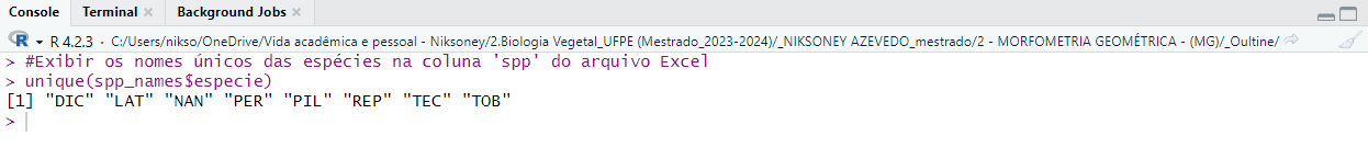
Step 4 - Build shape object
# Import coordinate data from text files
lf_coord <- import_txt(lf)

# Reorder coordinates to match Excel file order
lf_coord <- lf_coord[spp_names$individuo]

# Assign species names to coordinate objects
names(lf_coord) <- spp_names$especie

# Create factor variable for each individual
lf_fac <- as.data.frame(names(lf_coord))
names(lf_fac)[1] <- "Type"
lf_fac$Type <- as.factor(lf_fac$Type)

# Create Momocs Out object
lf_out <- Out(lf_coord, fac = lf_fac)
Step 5 - Visualize shapes and harmonics
# Save mean shapes plot
png("Imagens_prontas/formas_médias_esteril.png", width = 10, height = 8, units = "in", res = 300)
formas_gerais <- panel(lf_out, fac="Type", names=TRUE)
dev.off()
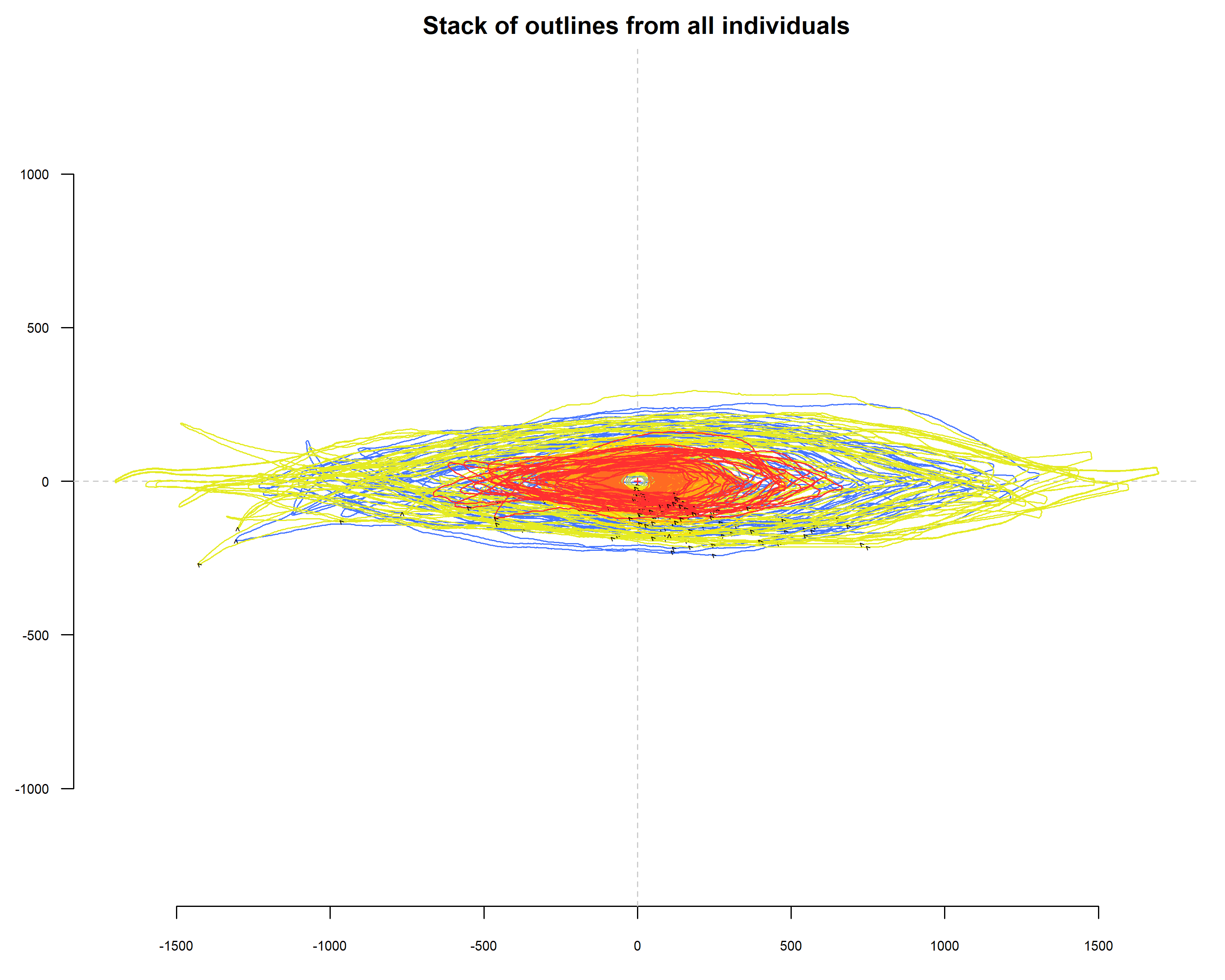
# Visualize contour stacks
stack(coo_center(lf_out),
palette = col_summer,
fac = lf_out$Type,
title = "Stack of outlines from all individuals",
subtitle = paste("Relação entre Área e Comprimento dos Contornos das Folhas"))
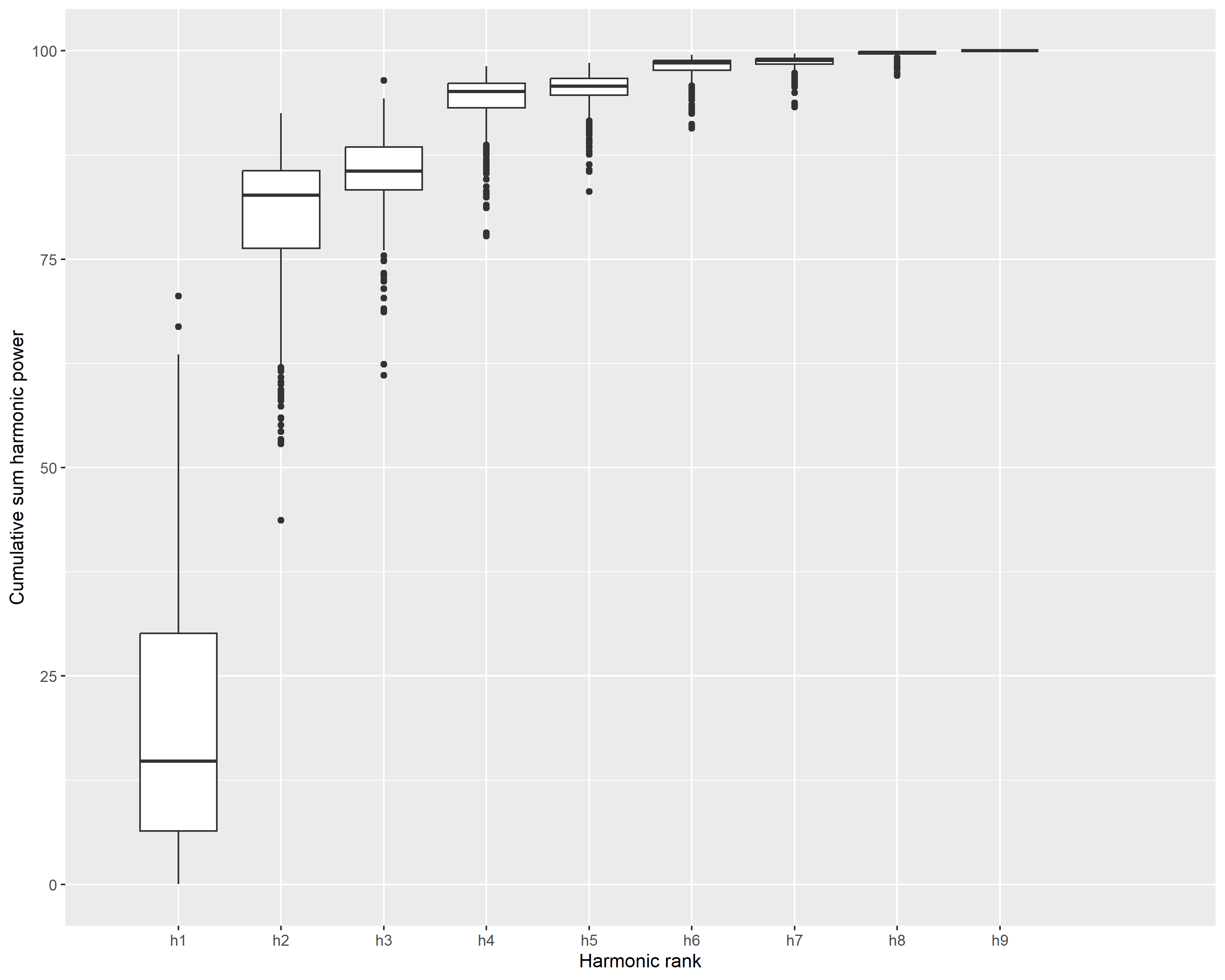
# Determine optimal number of harmonics
png("Imagens_prontas/harmonicos_esteril.png", width = 10, height = 8, units = "in", res = 300)
harmonics_info <- calibrate_harmonicpower_efourier(lf_out,
nb.h = 10,
drop = 1,
thresh = c(80, 90, 95, 99, 99.9),
plot = TRUE)
dev.off()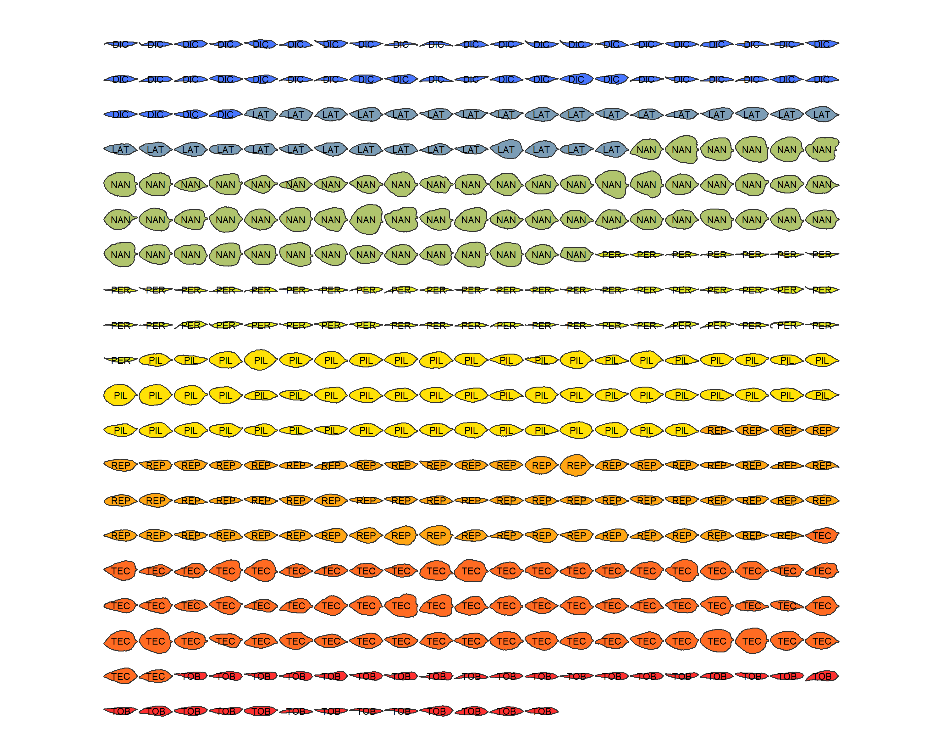
Step 6 - Run EFA
# Perform Elliptical Fourier Analysis
lf_fou <- efourier(x = lf_out,    # Shape coordinate data
                   nb.h = 8,      # Number of harmonics (from calibration)
                   norm = FALSE)   # No normalization
Step 7 - PCA and LDA analysis
# Principal Component Analysis
png("Imagens_prontas/pca_esteril_sproces.png", width = 10, height = 8, units = "in", res = 300)
lf_pca <- PCA(x = lf_fou, fac = lf_fou$fac)
plot_PCA(x = lf_pca, f = lf_pca$Type, palette = pal_manual(my_colors, transp = 0))
dev.off()
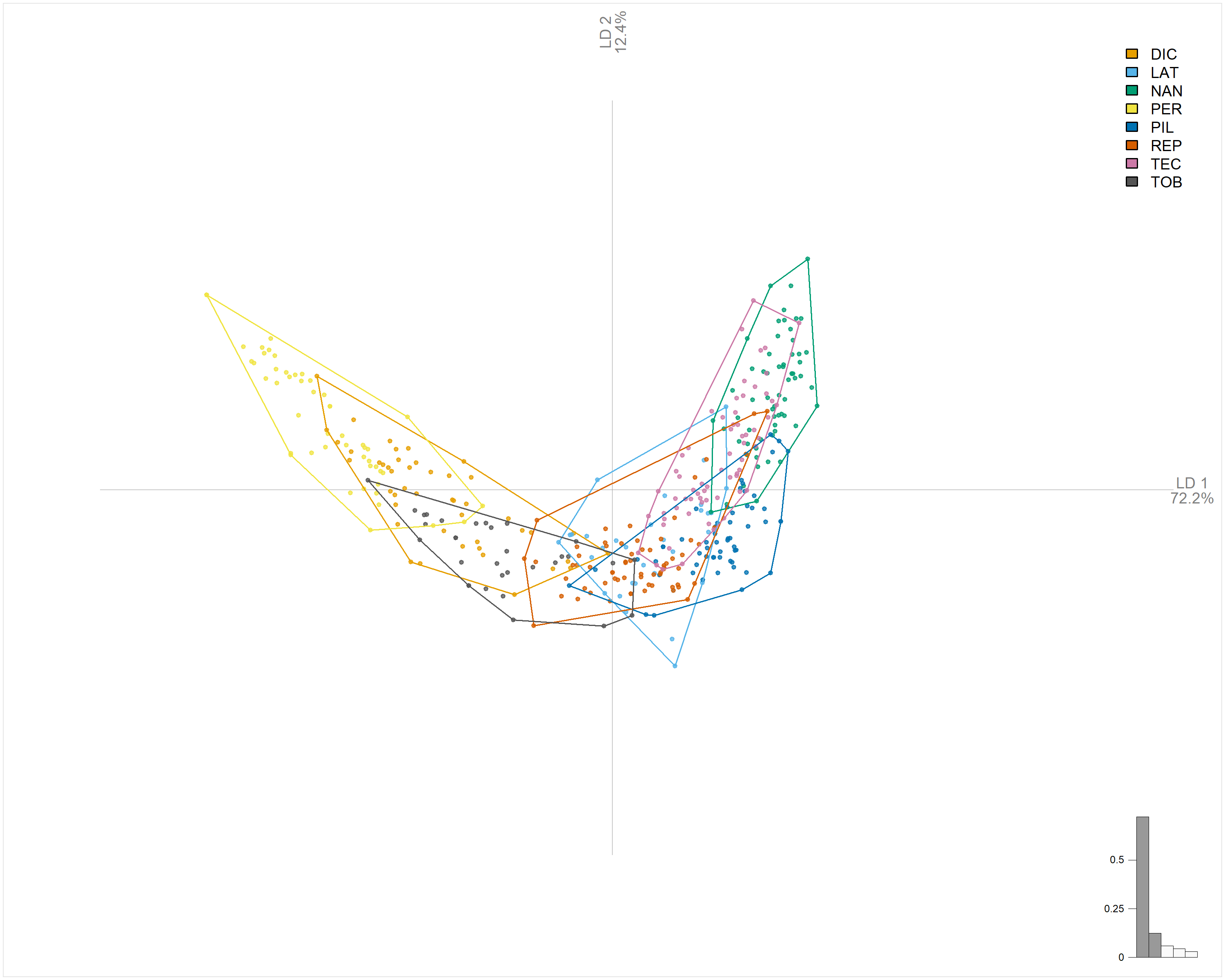
# Linear Discriminant Analysis
png("Imagens_prontas/lda_esteril_sproces.png", width = 10, height = 8, units = "in", res = 300)
lf_lda <- LDA(x = lf_fou, fac = lf_fou$Type)
plot_LDA(x = lf_lda, palette = pal_manual(my_colors, transp = 0))
# Check LDA accuracy
lf_fou %>% LDA(~Type) # 48% accuracy
dev.off()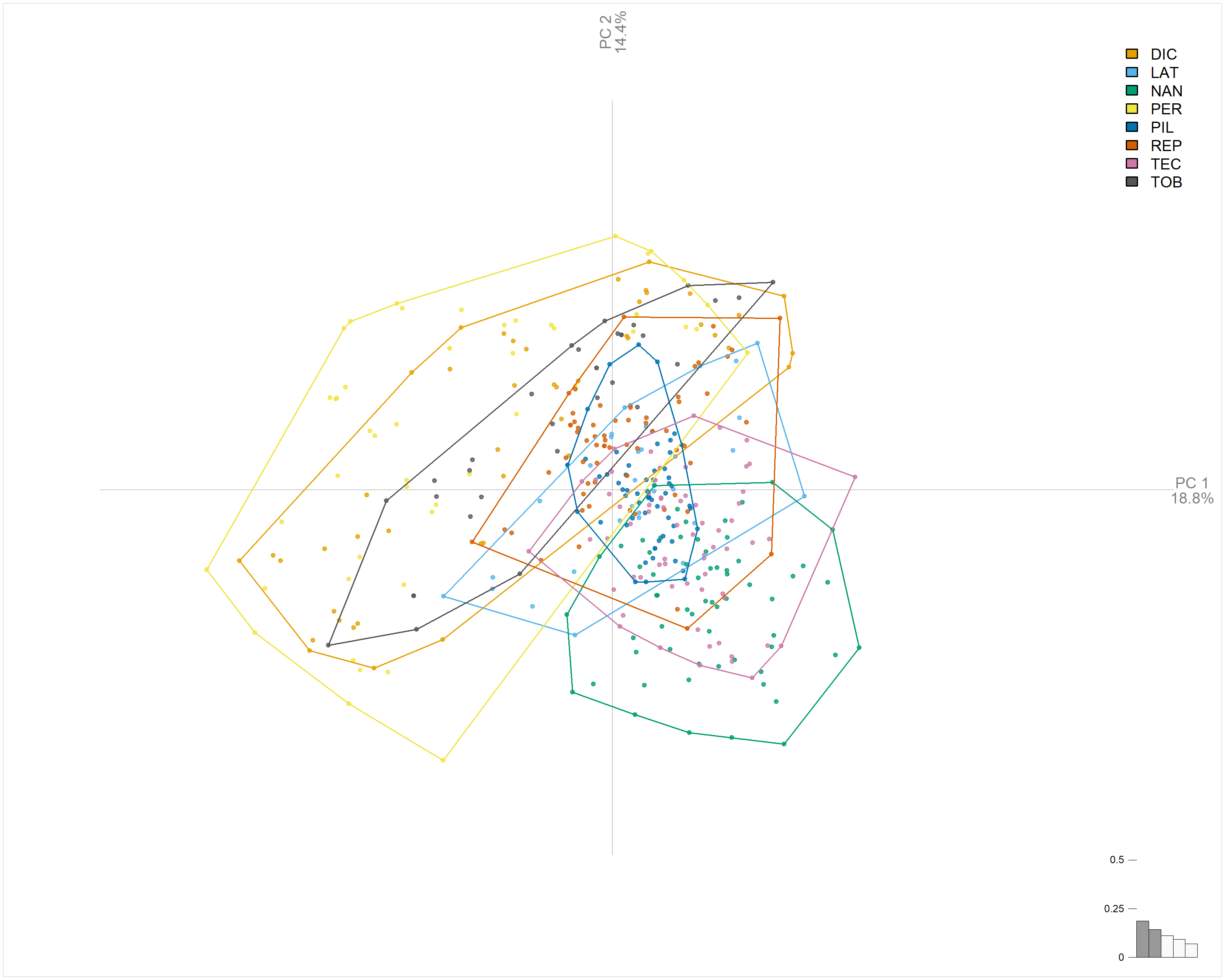
Pro Tips
Step 3: In the next step, remember to create an excel.xlsx file, in which one column must contain the same names as the species coordinate files.
Image resolution: Use 300 DPI for publication-quality figures.
Accessibility: Always include descriptive alt text for images.